Create Gantt Charts in Google Sheets: Auto-Update with Start and End Dates

2025年1月27日

Have you ever created a Gantt chart in a spreadsheet only to find yourself manually updating it every time you adjust task durations? It can be a tedious process, right?

With Google Sheets, you can use formulas and conditional formatting to create a Gantt chart that automatically updates whenever you change the start or end dates.

In this article, we’ll show you how to create an efficient Gantt chart using the “Project Tasks” template, helping you save time and streamline your project management.

For those using Google Workspace, you might also want to explore the “Timeline View” feature for an even more efficient way to create Gantt charts.

Example Output

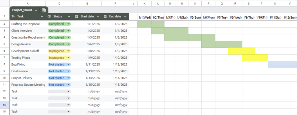
A Gantt chart is automatically created when you input the start and end dates.
Each task’s status (Not Started, In Progress, Completed) is color-coded for easy visual tracking.
Utilize the “Project Tasks” template in Google Sheets for a quick and effective setup.

Formulas Used

Automatically Populate Dates (Cell K1)

=IF(COUNTA(E2:E)=0, "", ARRAYFORMULA(MIN(FILTER(E2:E, E2:E<>"")) + SEQUENCE(1, MAX(FILTER(F2:F, F2:F<>"")) - MIN(FILTER(E2:E, E2:E<>"")) + 1, 0)))

This formula automatically generates a sequence of dates based on the earliest start date and the latest end date found in columns E and F.

Display Task Duration (Cell K2)

=ARRAYFORMULA(IF((($E2:$E<>"") * ($F2:$F<>"")) * (K$1:1 >= $E2:$E) * (K$1:1 <= $F2:$F), $D2:$D, ""))

This formula visually represents the task durations in the Gantt chart by comparing the task’s start and end dates with the dates in row K1, showing task names in their corresponding date range.

By combining the two formulas above with conditional formatting, you can create a functional Gantt chart.

Although the formulas are a bit lengthy, you can simply copy and paste them as-is to get started. (Detailed explanations for the formulas are provided in the step-by-step instructions.)

Steps to Create a Dynamic Gantt Chart in Google Sheets

STEP

Access the “Project Tasks” Template

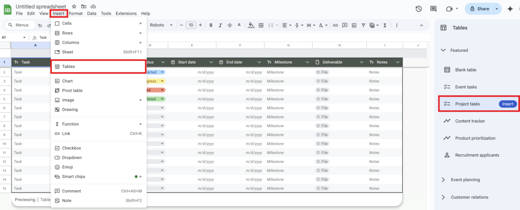
Open Google Sheets.

From the menu, click Insert and then select Table.

In the panel that appears on the right, choose the “Project Tasks” template to get started.

STEP

Input Data Fields

In the table, fill out the following columns:

Column A: Task Name (optional)
Column D: Status
Column E: Start Date
Column F: End Date

You can delete any other unnecessary columns after entering the formulas without affecting the functionality of the Gantt chart.

STEP

Enter the Formula to Automatically Generate Dates

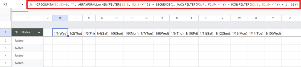
In cell K1, input the following formula:

=IF(COUNTA(E2:E)=0, "", ARRAYFORMULA(MIN(FILTER(E2:E, E2:E<>"")) + SEQUENCE(1, MAX(FILTER(F2:F, F2:F<>"")) - MIN(FILTER(E2:E, E2:E<>"")) + 1, 0)))

Formula Explanation

IF(COUNTA(E2:E)=0, "", ...)

Ensures that if there are no values in column E (Start Date), no dates are displayed.

ARRAYFORMULA

Processes the entire formula dynamically in one cell (K1), automatically generating dates without needing to copy it into multiple cells.

SEQUENCE

Generates a sequence of dates horizontally. The format SEQUENCE(1, number_of_columns) expands dates from the Start Date to the End Date across columns.

MIN(FILTER(E2:E, E2:E<>""))

Finds the earliest Start Date in column E.

The FILTER function excludes blank cells, ensuring only valid dates are considered.

MAX(FILTER(F2:F, F2:F<>""))

Finds the latest End Date in column F, ensuring the date range covers all tasks.

This formula uses the ARRAYFORMULA function to automatically display dates horizontally in row K and beyond.

The formula generates a range of dates starting from the earliest Start Date in column E to the latest End Date in column F.

With this formula, you create the horizontal axis, which serves as the foundation of your Gantt chart.

STEP

Generate the Gantt Chart

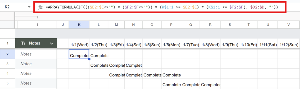
In cell K2, input the following formula:

=ARRAYFORMULA(IF((($E2:$E<>"") * ($F2:$F<>"")) * (K$1:1 >= $E2:$E) * (K$1:1 <= $F2:$F), $D2:$D, ""))

Formula Explanation

ARRAYFORMULA

processes the entire formula as an array, allowing it to calculate multiple rows of data simultaneously.

This eliminates the need to manually copy formulas into multiple cells, automating the process.

$E2:$E<>"" and$F2:$F<>""

Ensures that only rows where both the Start Date (column E) and End Date (column F) are not blank are processed.

Blank rows are ignored, keeping the formula efficient.

(K$1:1 >= $E2:$E) * (K$1:1 <= $F2:$F)

Checks the horizontal axis dates (starting from K1) against the task’s Start Date and End Date.

Conditions:

The date must be greater than or equal to the Start Date.
The date must be less than or equal to the End Date.

If both conditions are met, the corresponding cell in the Gantt chart will show a value.

$D2:$D

This is the value displayed in the cells that meet the conditions above.

In this case, it retrieves the status of the task from column D (e.g., “Not Started,” “In Progress,” “Completed”).

This formula also utilizes the ARRAYFORMULA function, so it automatically applies to all cells in row K2 and beyond.

Since this formula only displays the task status in the corresponding range, use Conditional Formatting to color-code the cells based on the task status (e.g., “Not Started,” “In Progress,” “Completed”). This step will visually transform the chart into a functional Gantt chart.

STEP

Apply Conditional Formatting for Color-Coding

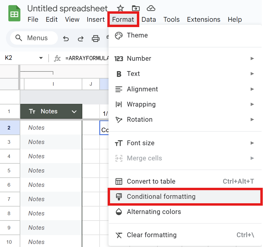
In the Google Sheets menu, click Format > Conditional formatting.

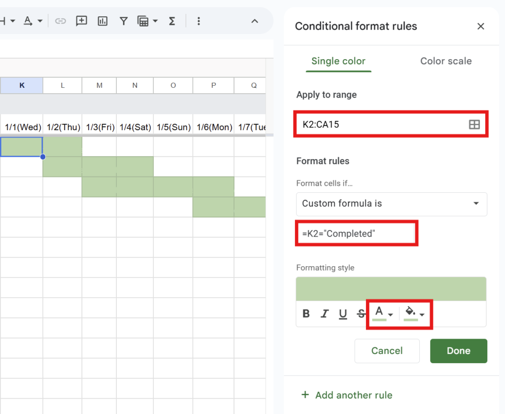
Define the Range to Apply Formatting

Select the entire range of the Gantt chart.

Example: K2:CA15

Set Conditional Formatting Rules

Select custom formulas to color-code each task.

For “Not Started”
- Custom Formula:=k2="Not Started"
- Text Color: Blue
- Fill Color: Blue
For “In Progress”
- Custom Formula:=k2="In Progress"
- Text Color: Yellow
- Fill Color: Yellow
For “Blocked”
- Custom Formula:=k2="Blocked"
- Text Color: Red
- Fill Color: Red
Completed
- Custom Formula:=k2="Completed"
- Text Color: Green
- Fill Color: Green

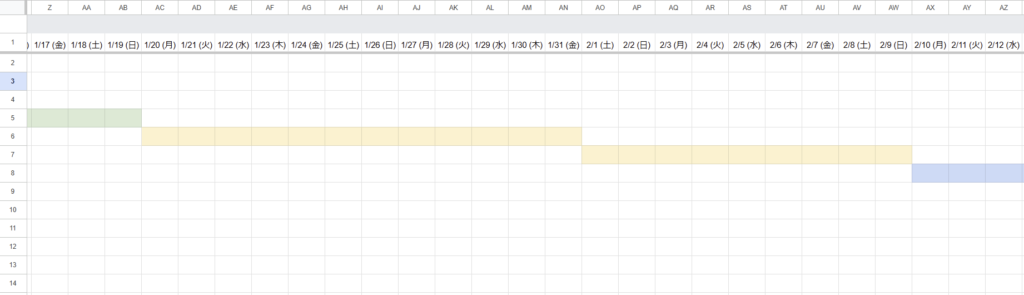
By setting the text color to match the fill color (e.g., blue text on a blue background), the text becomes invisible.

This creates a clean, visually appealing Gantt chart with only the colored blocks visible to represent task progress.

STEP

Final Touch

By changing the Start Date in column E or the End Date in column F, the Gantt chart will automatically update.

Conclusion

By using formulas and conditional formatting, you can create a dynamic Gantt chart in Google Sheets.

This method allows you to automatically update the chart by simply modifying the start and end dates, saving you the hassle of manual adjustments.

Feel free to use this approach whenever you need to create a Gantt chart in Google Sheets!

For managing multiple projects simultaneously or requiring more advanced features, consider using dedicated project management tools like Trello, Asana, or Jooto for even greater efficiency.