How to Identify Duplicate Data in Google Sheets: Using Functions and Conditional Formatting

In our previous article, we covered how to remove duplicate data in Google Sheets. This time, we’ll focus on how to extract duplicate data efficiently.

Using functions is ideal when you want to automate the extraction process, while conditional formatting is perfect for visually identifying duplicates at a glance. Both methods offer unique advantages depending on your specific needs.

あわせて読みたい

How to Identify Duplicate Data in Google Sheets: Using Functions and Conditional Formatting In our previous article, we covered how to remove duplicate data in Google Sheets. This time, we’ll focus on how to extract duplicate data efficiently. Using…

Extracting Duplicate Data Using Functions

There are two main methods to extract duplicate data using functions.

①Function to Display All Rows with Duplicate Data (FILTER and COUNTIF)

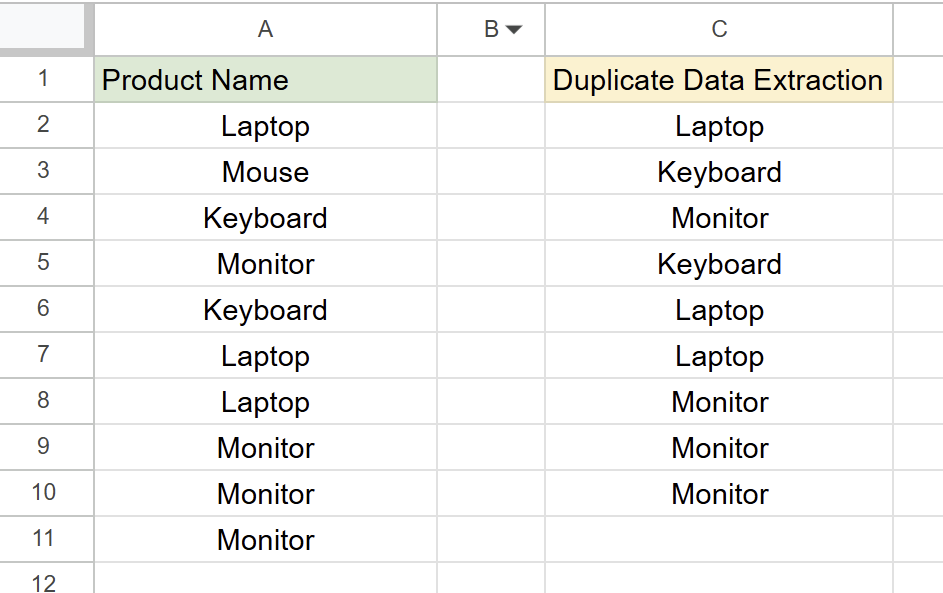
Example Formula:

=FILTER(A2:A, COUNTIF(A2:A, A2:A) > 1)

②Function to Display Duplicate Data Only Once (UNIQUE and FILTER)

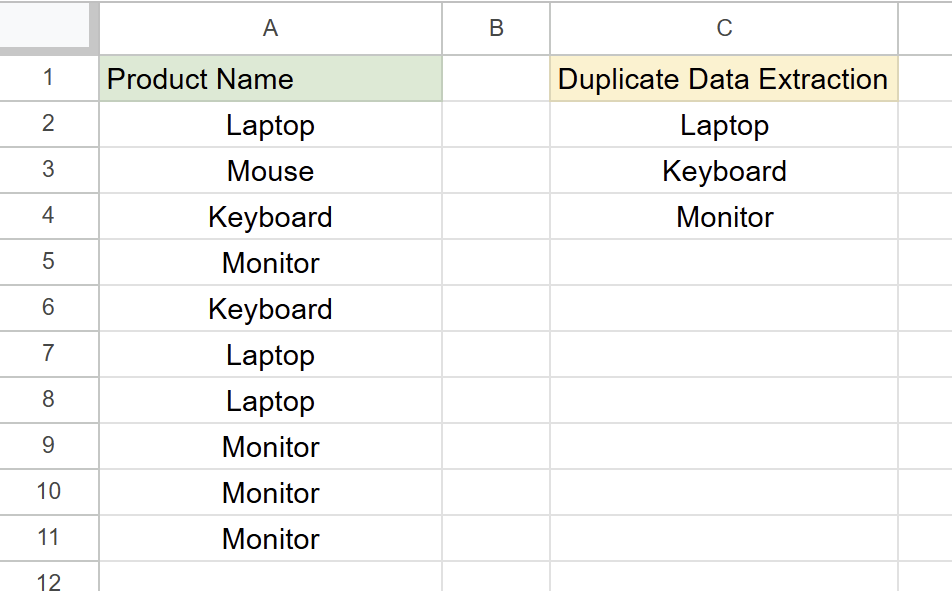
Example Formula:

=UNIQUE(FILTER(A2:A, COUNTIF(A2:A, A2:A) > 1))

To Display the Number of Duplicates for Each Data

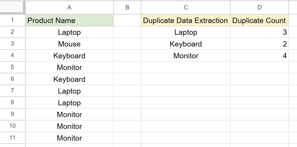
Example Formula to Show Duplicate Counts:

=ARRAYFORMULA(IF(C2:C <> "", COUNTIF(A:A, C2:C), ""))

Highlighting Duplicate Data Using Conditional Formatting

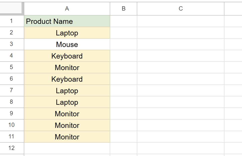
Conditional formatting is a convenient way to visually identify duplicate data.

STEP

Select the Data Range

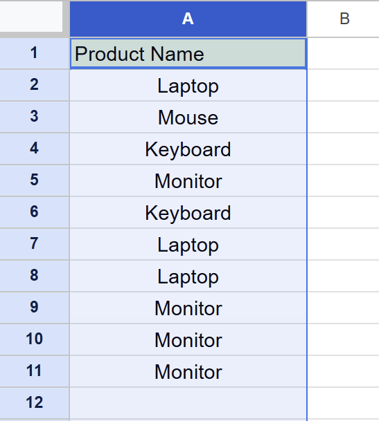
Choose the range of data where you want to find duplicates.

STEP

Open Conditional Formatting

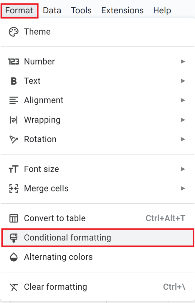
From the menu, select “Format” → “Conditional formatting.”

(You can also right-click and select “Conditional formatting” from the context menu.)

STEP

Choose Custom Formula

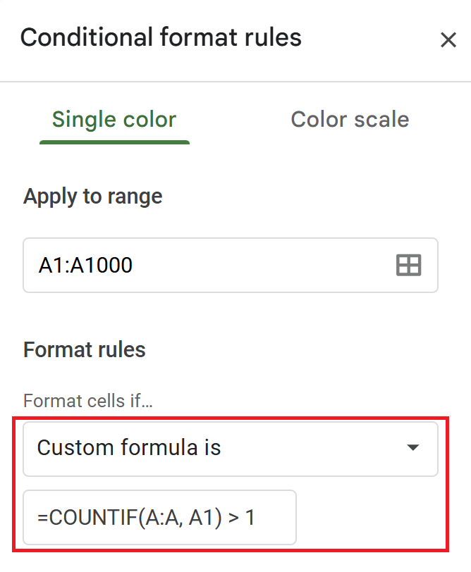
In the conditional formatting rules, select “Custom formula is” and enter the following formula.

Example Formula (to check column A):

=COUNTIF(A:A, A1) > 1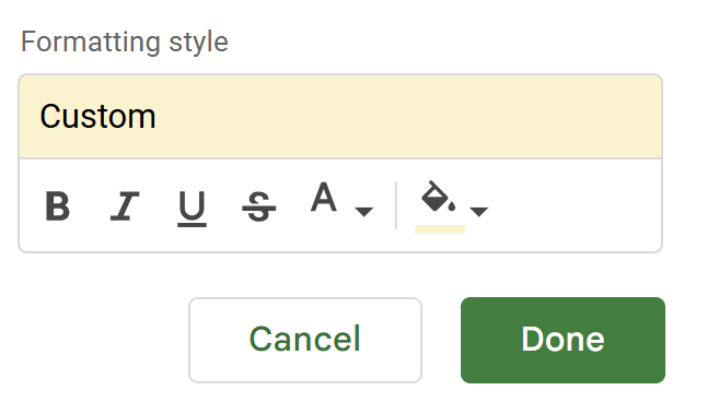

STEP

Select the Desired Color and Finish

Choose your preferred color for highlighting and click “Done” to apply the formatting.

Conclusion

There are several methods to extract duplicate data in Google Sheets, including using functions and conditional formatting.

For more advanced customization, you can also use Google Apps Script (GAS) to extract duplicate data.

Choose the method that best fits your specific needs to streamline your workflow effectively.

• Functions: When you want to automatically filter duplicates.
• Conditional Formatting: When you need to visually identify duplicates.
• GAS (Google Apps Script): When customized processing is required.

あわせて読みたい

How to Identify Duplicate Data in Google Sheets: Using Functions and Conditional Formatting In our previous article, we covered how to remove duplicate data in Google Sheets. This time, we’ll focus on how to extract duplicate data efficiently. Using…